Why 1×32 is the default choice - and where that logic runs out
The capital-expenditure case for 1×32 is real. One OLT port, one feeder fiber, one splitter, thirty-two subscribers. Compare that to deploying two 1×16 units: a second OLT port, a second feeder run, more cabinet space. At per-port pricing, the 1×32 option commonly appears 30–40% cheaper on the line-item budget before a trench is opened. For a rollout covering hundreds of distribution points, that arithmetic adds up to a significant capex difference.
Network planners add a second argument: unused ports on a 1×32 absorb future subscribers without a new unit. A filled 1×16 requires a second device, a second OLT port, and a truck roll. The 1×32 looks like it defers future cost.
Both arguments hold - when the optical budget also holds. What the budget spreadsheet doesn't automatically capture is where optical power actually goes as it travels from an OLT through 8 km of feeder cable, through a splice closure, through a 1×32 splitter, through a FAT adapter, down a drop cable, and into an ONT receiver on a cold morning when the aerial closure is sitting at −3 °C. That path adds loss that no datasheet anticipates on your behalf.
What 1×32 actually costs in decibels - and what gets added on top
If you need a refresher on how splitting loss is calculated from first principles, our main guide covers the full derivation: How Fiber Splitters Work: Physics, Types, Loss Budgets & Design. The short version for planning purposes: a 1×32 split has a theoretical floor of 15.05 dB, and real PLC devices add 1.0–2.5 dB of excess loss above that floor - giving a maximum insertion loss of 17.5 dB under the ITU-T G.984 spec.
The number that matters for deployment decisions is not the theoretical floor; it is the spread between the datasheet maximum and what you actually get after installation. A well-manufactured PLC 1×32 unit, produced under controlled conditions with 100% per-unit testing, typically lands around 16.7–16.9 dB mean IL - roughly 0.6–0.8 dB below the spec ceiling. A commodity unit sourced without per-unit testing may arrive anywhere within the 17.5 dB limit, or occasionally over it. On a Class B+ link with 3 dB of aging margin, that variance is the difference between a design that ages gracefully and one that needs a maintenance intervention by year five.
| Split ratio | Theoretical split loss | Typical max IL (spec) | Best-in-class max IL | Uniformity (max) |
|---|---|---|---|---|
| 1×2 | 3.0 dB | 3.6 dB | 3.4 dB | ≤0.6 dB |
| 1×4 | 6.0 dB | 7.4 dB | 7.0 dB | ≤0.8 dB |
| 1×8 | 9.0 dB | 11.0 dB | 10.5 dB | ≤1.0 dB |
| 1×16 | 12.0 dB | 14.0 dB | 13.5 dB | ≤1.4 dB |
| 1×32 | 15.0 dB | 17.5 dB | 16.8 dB | ≤1.9 dB |
| 1×64 | 18.0 dB | 21.0 dB | 20.5 dB | ≤2.5 dB |
The "best-in-class" column matters. A 1×32 unit from a manufacturer running 100% per-unit IL/RL testing and tight process control can deliver 16.8 dB mean insertion loss - roughly 0.7 dB below the 17.5 dB spec ceiling. That 0.7 dB is not marketing; it is engineering headroom. At 0.35 dB/km of feeder cable it represents two additional kilometers of reach, or the absorption of two marginal field splices before the budget breaks.
Class B+ vs C+ - what the OLT class actually changes
The ITU-T G.984 GPON standard defines attenuation classes that set the total allowed budget between OLT and ONT. The two classes that dominate ISP procurement are:
- Class B+: 13–28 dB total attenuation budget (net budget: 28 dB)
- Class C+: 17–32 dB total attenuation budget (net budget: 32 dB)
The difference is 4 dB - which sounds small until you map it against a full link budget. Here are two worked examples: a 1×32 deployment on Class B+ versus Class C+, both at 8 km of feeder cable.
This table reveals the decision that most deployment guides skip entirely: the OLT class matters as much as the splitter spec. A 1×32 splitter on a Class B+ OLT at moderate cable distances is a marginal design on day one. The same splitter on a Class C+ OLT is conservative engineering. The device is identical; the system context is not.
Where most FTTH power budgets actually break
If you ran a postmortem on every FTTH link that failed its loss budget in the first three years of service, the cause distribution would look approximately like this - based on field-service data and engineering community discussions from NANOG, ISE Magazine, and independent ISP forums:
| Root cause | Estimated share of failures | Typical dB impact |
|---|---|---|
| Dirty or damaged APC connector endface | ~40% | 0.5–3.0 dB per connector |
| Installed IL higher than max spec (inferior splitter) | ~20% | 0.5–2.0 dB |
| Aging margin not included in design budget | ~15% | 1.5–3.0 dB accumulated |
| Field-splice quality below design assumption | ~12% | 0.1–0.5 dB per splice |
| APC/UPC connector mismatch in drop path | ~8% | 0.3–1.5 dB + return-loss collapse |
| Actual fiber cable loss higher than spec | ~5% | 0.05–0.1 dB/km above 0.35 |
The pattern that jumps out: the splitter's intrinsic insertion loss is responsible for roughly 20% of failures, almost always because a commodity unit was sourced without per-unit testing and its "1×32 ≤ 17.5 dB" label conceals an actual installed loss of 18.5–19 dB. The other 80% of failures are in the path around the splitter - connectors, splices, design margin, and connector-type mismatches.
The three loss events that kill more links than any splitter spec
1. Connector contamination at the splitter pigtail
The output pigtails of a 1×32 cassette splitter each end in an SC/APC connector. Each of those 32 connectors is a potential contamination site. A single 9 µm single-mode APC endface with a debris particle on the fiber core can add 0.5–3 dB of insertion loss - the equivalent of swapping a high-grade splitter for a commodity one. In a 1×32 unit, you have 33 connector interfaces (one input, 32 outputs) where this can happen. Field inspection with a fiber endface scope before every mating is not optional; it is the single highest-leverage action in field quality control.
2. Field-splice performance versus design assumption
Loss budgets routinely assume 0.1 dB per fusion splice. A skilled technician with a calibrated fusion splicer achieves 0.05–0.08 dB per splice under controlled conditions. In a distribution closure on a windy afternoon, the same technician with the same splicer might achieve 0.15–0.3 dB per splice because fiber alignment varies with handling. Four splices at 0.25 dB each instead of 0.1 dB each adds 0.6 dB of unbudgeted loss - which consumes 20% of the aging margin in the worked example above.
3. The "missing" aging margin
Network components degrade. Connector mating surfaces develop wear facets. Epoxy joints in fusion closures creep under thermal cycling. Outdoor enclosure seals allow micro-moisture ingress. Over 25 years, a well-engineered network accumulates 1.5–3 dB of loss beyond commissioning values. A budget that closes to within 1 dB on commissioning day will not close in year eight. APNIC's published GPON budget analysis confirms that inaccurate or optimistic loss calculations are among the leading causes of in-service receiver problems in deployed FTTx systems.
1×16 vs 1×32 in real deployment scenarios
The right split ratio is not a global answer - it is the answer to a topology question. Here are four deployment types with the engineering recommendation for each, derived from field experience and the loss-budget arithmetic above.
The suburban scenario is the one that generates the majority of field problems. It is common, it is where Class B+ OLTs are routinely deployed, and it is exactly the topology where 1×32 and 1×16 look interchangeable on a spreadsheet but produce very different outcomes over ten years of operation.
Why many operators prefer cascaded splitting - and its real cost
Centralized splitting puts one 1×32 unit in a fiber distribution hub, and 32 fibers fan out to 32 ONTs. Cascaded splitting places a 1×4 unit near the OLT and four 1×8 units closer to the subscribers. The result is still 32 outputs, but the optical path is different.
The loss math on cascaded vs. centralized 1×32
| Architecture | Splitter loss | Extra splice points | Total splitter + splice overhead |
|---|---|---|---|
| Centralized 1×32 | 17.5 dB (max) | 0 extra | 17.5 dB |
| Cascaded 1×4 + 1×8 | 7.4 + 11.0 = 18.4 dB | +4 splice joints | 18.4 + 0.4 = 18.8 dB |
| Cascaded 1×2 + 1×16 | 3.6 + 14.0 = 17.6 dB | +2 splice joints | 17.6 + 0.2 = 17.8 dB |
Cascaded splitting costs you 0.9–1.3 dB more loss versus centralized on an equivalent subscriber count - the physics of stacking split events is unavoidable. So why do experienced operators choose it?
The legitimate case for cascaded splitting
- Feeder fiber savings. In a rural or semi-rural deployment, the distance from OLT to a distribution point may be 10–15 km, but each subscriber is only 200–500 m from that distribution point. Running 32 individual drop fibers over 10 km is far more expensive than running one feeder to the distribution point and 32 short drops from there. Cascaded splitting allows that topology.
- Staged build-out. A 1×4 unit at the OLT can initially feed only two 1×8 splitters; the other two ports remain capped until subscriber density grows. This is impossible with a single 1×32 unit committed to a specific location.
- Fault isolation. A fault in one 1×8 stage affects only 8 subscribers. A fault in the single 1×32 affects all 32. For SLA-heavy commercial deployments, this matters.
How to calculate a safe GPON margin - the step-by-step method
Safe margin is not a guess; it is a calculation. Here is the method as practiced by experienced ODN engineers, applied to a 1×32 deployment on a Class B+ OLT at 10 km.
Step 1 - Establish the gross budget
Gross budget = OLT Tx power − ONT Rx sensitivity. For GPON Class B+: +3 dBm Tx, −28 dBm Rx sensitivity → 28 dB gross budget. For Class C+: +5 dBm Tx, −32 dBm Rx → 32 dB gross budget. Always use the maximum insertion loss value from the worst receiver sensitivity on the datasheet - not typical.
Step 2 - Sum all fixed losses
- Fiber attenuation: total route length (km) × 0.35 dB/km at 1490 nm for G.652D cable. Use the cable vendor's actual spec; do not assume the ITU floor.
- Splitter insertion loss: maximum IL from the datasheet, not typical. For our 1×32: 17.5 dB max (or 16.8 dB if ordering units with per-unit certificates).
- Connector mating loss: 0.3 dB per mating in field conditions. Count every connector interface: OLT patch panel, splitter input, splitter output, FAT adapter, ONT drop connector. A typical 1×32 link has 6–8 mating points.
- Splice loss: 0.1 dB per fusion splice (well-executed field splice). Count every splice in the route.
Step 3 - Reserve aging and repair margin
This is the step most failed budgets skip. Allocate a minimum of 3 dB for aging and repair margin. This covers: connector surface wear over 15+ years (~0.5 dB), epoxy joint creep and moisture ingress (~0.5 dB), two future repair splices replacing factory-quality splices (~0.4 dB), and a buffer for one connector replacement on the ONT drop side (~0.5 dB). The remaining ~1 dB covers temperature excursion and measurement uncertainty. Three decibels is not padding - it is amortized field reality.
Step 4 - Check margin; adjust if needed
If (gross budget − fixed losses − aging margin) ≥ 0, you have a valid design. If the remainder is negative or below 1 dB, you have three levers: upgrade OLT class (adds 4 dB), reduce split ratio from 1×32 to 1×16 (saves 3.5 dB), or shorten the cable route. Changing connector quality from generic (0.5 dB) to best-grade APC (0.3 dB) on eight interfaces saves 1.6 dB - often enough to rescue a borderline design.
XGS-PON changes the equation - but not the math
XGS-PON (ITU-T G.9807.1) delivers 10 Gbps symmetrically and introduces its own attenuation classes: N1 (29 dB budget), N2 (31 dB budget), and E1 (35 dB budget). The splitter physics is identical - a 1×32 PLC unit still costs 17.5 dB max - but the available headroom shifts significantly, and the wavelength plan changes.
XGS-PON downstream operates at 1577 nm rather than GPON's 1490 nm. G.652D single-mode fiber has slightly lower attenuation at 1577 nm (~0.30 dB/km versus ~0.35 dB/km at 1490 nm). On a 10 km link, that difference is 0.5 dB - modest, but measurable when budgets are tight. More significantly, XGS-PON's N2 class at 31 dB matches GPON Class C+ very closely, making most C+ plant directly compatible with XGS-PON N2 OLT upgrades without re-engineering the ODN.
| Standard | Class | Gross budget | Non-splitter loss (typical) | Headroom after 1×32 | Verdict |
|---|---|---|---|---|---|
| GPON | Class B+ | 28 dB | ~7.0 dB | 3.5 dB | Marginal at 8 km |
| GPON | Class C+ | 32 dB | ~7.0 dB | 7.5 dB | Comfortable |
| XGS-PON | N1 | 29 dB | ~6.5 dB (lower fiber loss) | 5.0 dB | Adequate |
| XGS-PON | N2 | 31 dB | ~6.5 dB | 7.0 dB | Comfortable |
| XGS-PON | E1 | 35 dB | ~6.5 dB | 11.0 dB | Suitable even for 1×64 |
The practical takeaway: operators planning an eventual migration from GPON to XGS-PON should ensure the existing ODN is built to at least Class C+ standards. A 1×32 plant designed to Class B+ limits may require OLT-class upgrades or split-ratio reduction when XGS-PON is introduced - because higher-class XGS-PON OLTs are needed to maintain reach parity. Our PLC splitter range (1×2 to 1×64) covers all GPON and XGS-PON wavelength plans with a flat 1260–1650 nm response, avoiding a hardware swap when the OLT generation changes.
Frequently asked questions
-
Q: What is the typical insertion loss of a 1×32 splitter?
A: The ITU-T G.984-aligned specification for a 1×32 PLC splitter is a maximum insertion loss of 17.5 dB at 1260–1650 nm, with port-to-port uniformity of ≤1.9 dB. Well-manufactured units tested on 100% of production achieve mean insertion loss of 16.7–16.9 dB - approximately 0.7 dB below the spec ceiling. Always design to the maximum, never to the typical, because field conditions add loss that the lab does not.
Q: Is 1×64 practical for GPON?
A: Yes, but only under specific conditions: GPON Class C+ or higher OLT, feeder cable under 3–4 km, high-quality fusion splicing throughout, and per-unit acceptance testing on the splitter. A 1×64 PLC unit has a maximum insertion loss of 21 dB. On a Class B+ OLT with a 28 dB gross budget, after fiber and connector losses you have essentially no aging margin. The ITU-T G.984 standard acknowledges 1×64 for Class C+ networks specifically. In practice, 1×64 is the standard choice for high-density urban MDU deployments in Europe (OpenFiber, FiberCop) where route distances are short and OLT classes are high. It is rarely the right answer for suburban or rural builds.
Q: How much reserve margin should FTTH networks keep?
A: A minimum of 3 dB aging and repair margin is the standard recommendation from field engineering practice. This accounts for connector wear, joint creep, future repair splices, and measurement uncertainty over a 25-year network life. Networks designed without explicit aging margin routinely require unplanned OLT upgrades or splitter replacements within 5–8 years of commissioning. If your topology forces a budget under 3 dB margin, upgrade the OLT class or reduce the split ratio - do not accept the thin margin.
Q: Does cascaded splitting increase failure rate?
A: Not intrinsically - a PLC chip is a PLC chip regardless of where it sits in the cascade. Cascaded splitting does introduce more splice points and connector interfaces, each of which is a potential contamination or mechanical failure site. It also makes fault isolation harder: when a 1×8 stage fails in a cascade, you lose 8 subscribers; the fault could be in the 1×4 first-stage pigtail or in the 1×8 unit, requiring OTDR work from multiple access points. Whether that operational complexity justifies the feeder fiber savings depends on route geometry and crew cost in your market.
Q: When should I use 1×16 instead of 1×32?
A: Use 1×16 when: your OLT is Class B+ (28 dB budget), your feeder cable exceeds 8 km, your link operates in harsh outdoor conditions that demand extra aging margin, or your fiber plant uses connector quality below APC-grade. The 3.5 dB difference between 1×32 (17.5 dB max) and 1×16 (14.0 dB max) translates directly into reach, aging headroom, or the ability to absorb a below-spec field repair without a service call. On Class C+ OLTs and routes under 5 km, 1×32 is generally the better economic choice.
Q: Can I mix 1×32 and 1×16 splitters in the same PON tree?
A: No - a single PON tree means all ONTs share the same OLT port and therefore the same downstream signal path to the primary splitter. You cannot have different split ratios in parallel from the same input fiber unless you are using cascaded splitting, where a 1×N first stage feeds different second-stage split counts. In a two-stage cascade, different second-stage ratios are technically possible (one 1×8 and one 1×4 feeding from the same 1×4 first stage, for example), but they produce different insertion-loss paths to different subscribers - which complicates fault diagnosis and OTDR interpretation significantly.
- ITU-T G.984.1 - GPON General Characteristics (attenuation classes B+, C+, C++)
- ITU-T G.9807.1 - XGS-PON 10 Gbps symmetrical (classes N1, N2, E1)
- Telcordia GR-1209 / GR-1221 - Generic reliability criteria for passive optical components (environmental, mechanical, aging)
- The Fiber Optic Association (FOA) - Guidelines on what loss to expect when testing fiber optic cables
- APNIC Blog - GPON Power Budget Calculations (2024)