
What a Fiber Splitter actually is
A fiber optic splitter is a passive optical component that takes one incoming light signal and divides it among two or more output fibers - or, run in reverse, combines several inputs into one. Unlike active devices that need electricity, a splitter relies only on the behavior of light inside glass, which is what makes it cheap to deploy and reliable in places you cannot easily power or reach.
That single property - passivity - is the reason the entire passive optical network (PON) architecture exists. One fiber leaves a central office, hits a splitter, and serves dozens of homes. There is no powered equipment between the Optical Line Terminal (OLT) and the subscriber's Optical Network Terminal (ONT). The splitter is the component that makes "one fiber, many customers" physically possible.
The physics: how one beam of light becomes many
Light stays inside an optical fiber because of total internal reflection. The glass core has a slightly higher refractive index than the surrounding cladding, so when light strikes that boundary at a shallow enough angle, it reflects back into the core instead of leaking out. Guide that light into a structure where the boundary geometry changes, and you can force the energy to redistribute into multiple paths. That is the whole trick.
There are two ways to build that structure, and they correspond to the two splitter families you will buy.

FBT vs PLC: two ways to build the same function
Fused Biconical Taper (FBT)
The older method. Two or more bare fibers are aligned, then heated and stretched on a tapering machine until their cores fuse into a single coupling region. As light enters that tapered zone it couples across into the adjacent fiber cores, and at the end of the taper the power exits split between the outputs. The stretch length and twist angle set during manufacturing determine the ratio. FBT is inexpensive and lets you build asymmetric ratios (say 5/95 or 30/70 taps), but precision falls off fast: above a 1×8 split it must be assembled from cascaded 1×2 units, and the failure rate climbs.
Planar Lightwave Circuit (PLC)
The modern method for high counts. Waveguides are etched onto a silica or silicon chip using photolithography - the same class of process used to make semiconductors. Light enters one waveguide and splits at precisely defined Y-branches into 4, 8, 16, 32, or 64 outputs. Because the geometry is lithographically defined rather than hand-pulled, PLC splitters deliver uniform loss across all ports and a flat response from 1260 to 1650 nm - covering every PON wavelength in one device.
| Parameter | FBT splitter | PLC splitter |
|---|---|---|
| Build | Fused, stretched fibers | Etched waveguide chip |
| Practical split ceiling | 1×8 (higher = cascaded, higher failure) | 1×64 in a single device |
| Wavelength range | Fixed windows (1310/1490/1550 nm) | 1260–1650 nm, flat |
| Port-to-port uniformity | Variable | Tight |
| Temperature loss drift (TDL) | ~0.5 dB/°C | ~0.2 dB/°C |
| Operating temperature | −5 to +75 °C | −40 to +85 °C |
| Best use | 1×2/2×2 taps, asymmetric ratios, monitoring | FTTH/PON distribution, 1×8 and above |
Why splitting always costs you decibels
This is the part most "how it works" articles skip, and it is the part that decides whether your network functions. When you divide optical power N ways, each output can only receive a fraction of the input. The unavoidable, physics-floor loss for an even split is:
Theoretical split loss (dB) = 10 × log₁₀(N)
So a 1×2 split loses at least 3 dB, a 1×4 loses 6 dB, a 1×8 loses 9 dB, and so on. Real devices lose more than this, because of excess loss - the energy lost to scattering, imperfect coupling, and material absorption inside the device. The number you actually design with is insertion loss, which folds the theoretical split and the excess loss together.
| Split ratio | Theoretical split loss | Typical max insertion loss | Loss uniformity |
|---|---|---|---|
| 1×2 | 3.0 dB | 3.6 dB | ≤0.6 dB |
| 1×4 | 6.0 dB | 7.4 dB | ≤0.8 dB |
| 1×8 | 9.0 dB | 11.0 dB | ≤1.0 dB |
| 1×16 | 12.0 dB | 14.0 dB | ≤1.4 dB |
| 1×32 | 15.0 dB | 17.5 dB | ≤1.9 dB |
| 1×64 | 18.0 dB | 21.0 dB | ≤2.5 dB |
The specs that catch people out
Insertion loss gets all the attention, but three other numbers decide reliability:
- Uniformity - the spread between the best and worst output port on a single device. A 1×32 with poor uniformity means some subscribers run close to the budget edge while others have margin to spare.
- Return loss (RL) - reflected light coming back toward the source. Higher is better; APC connectors give ≥60 dB versus ~50 dB for UPC, which is why PON drops almost always use APC.
- Polarization-dependent loss (PDL) and temperature-dependent loss (TDL) - small in PLC (≈0.1–0.2 dB), but in FBT the temperature drift alone can push a marginal link out of budget on a cold night.
A worked example: closing a real loss budget
Specs only matter when you add them up. Here is the calculation an engineer runs before ordering a single splitter. Assume a GPON downstream with a +3 dBm OLT launch and an ONT receiver sensitivity of −28 dBm - giving a total budget of 31 dB.
| Element | Loss | Running total |
|---|---|---|
| OLT launch power | +3.0 dBm | - |
| Feeder + drop fiber, 8 km @ 0.35 dB/km | 2.8 dB | 2.8 dB |
| 1×32 PLC splitter insertion loss | 17.5 dB | 20.3 dB |
| Connectors (4 × 0.3 dB) | 1.2 dB | 21.5 dB |
| Splices (4 × 0.1 dB) | 0.4 dB | 21.9 dB |
| Aging / repair margin | 3.0 dB | 24.9 dB |
| Power at ONT | +3.0 − 24.9 = −21.9 dBm - inside the −28 dBm limit ✓ | |
The splitter alone consumes more than 70% of the spent budget in this design. That single fact drives almost every architectural decision in PON. It is also why a poorly specified splitter - one whose "1×32" is really 18.5 dB instead of 17.5 dB - can quietly eat your entire repair margin before a technician ever touches the cable.
Centralized vs cascaded splitting
Once you know the loss math, the deployment choice follows. There are two ways to reach, say, 32 homes.
Centralized: a single 1×32 splitter sits in a fiber distribution hub, and 32 fibers fan out to 32 ONTs. One splitter, one loss event (~17.5 dB), easy to test and monitor. This is the standard choice in dense urban areas because access is easy and you can leave splitter ports unused until subscribers sign up.
Cascaded: a 1×4 splitter in an outside enclosure feeds four 1×8 splitters closer to the customers. The result is still 32 outputs, but the loss now stacks: roughly 7.4 dB (1×4) + 11 dB (1×8) ≈ 18.4 dB - about a decibel worse than centralized. The payoff is far less feeder fiber, which is why cascaded splitting wins in spread-out rural or village routes where fiber length, not access, is the cost driver.
Field troubleshooting: the splitter is rarely the culprit
When a link reads high loss, the splitter takes the blame and gets swapped first. It is almost always the wrong move. Insertion loss is the sum of every connector, splice, bend, and component in the path, and the reading at the endpoint tells you nothing about where the loss lives. Before condemning a splitter:
- Inspect and clean every endface. A single contaminated APC connector can add more loss than a poorly performing splitter. Clean with anhydrous ethanol and a lint-free wipe before measuring.
- Check your reference. A 1 dB error in your OTDR or power-meter reference launch shows up as 1 dB of phantom splitter loss.
- Confirm wavelength. A device measured at 1550 nm reads differently than the 1490 nm downstream it actually carries; a mismatch fakes a problem.
- Account for the cascade. If you forgot a second splitter stage in your budget, the link is doing exactly what physics says - your spreadsheet is wrong, not the hardware.
Only after those four checks does swapping the splitter make sense. Most "bad splitter" calls resolve at step one.
6 real-world pitfalls - mistakes engineers keep making
Theory is clean; field installs are not. The six failure patterns below appear repeatedly in ISP forums, NANOG mailing-list archives, and industry field-service reports. None of them require exotic hardware to trigger - they all happen with ordinary decisions made in a hurry.
Standards and what compliance actually guarantees
A splitter that closes the budget on day one but fails after three winters is worthless. That is what the standards address. Two bodies matter:
- ITU-T G.984 (GPON) defines the optical link budgets - the attenuation classes (Class B+ at 13–28 dB, Class C+ at 17–32 dB) that your splitter loss has to fit inside. This is the spec that tells you whether a 1×64 is even legal on a given OLT.
- Telcordia GR-1209 and GR-1221 set the generic reliability criteria for passive optical components - the environmental, mechanical, and aging tests (including the damp-heat and thermal cycling that an FTTH network has to survive over its 25-year life).
When a splitter datasheet cites GR-1209/GR-1221, it is claiming the device passed accelerated-aging and environmental qualification - not just that it measured well once on a bench. For outdoor and aerial deployments, that distinction is the entire point. Glory Optical manufactures under an ISO 9001:2015 quality system with full batch traceability, and validates optical and environmental performance in-house against IEC, ITU-T, and Telcordia criteria.
Where this is heading
Splitter demand tracks fiber rollout, and fiber rollout is accelerating. The splitter segment of the passive optical component market is forecast to grow at roughly a 15% CAGR through 2030, driven by FTTH build-out, 5G fronthaul, and hyperscale data centers. The technical pressure is toward higher split counts (1×64 and beyond) at flatter loss, and toward devices rated for the newer XGS-PON and NG-PON2 wavelength plans rather than GPON alone. In practice that means PLC continues to displace FBT for distribution, while FBT holds its niche in monitoring taps and asymmetric couplers. The component does not change much; the budgets it has to fit inside keep getting tighter.
Frequently asked questions
-
Q: How does a fiber splitter work without power?
A: It exploits total internal reflection inside glass. Light entering the device is guided through a fused coupling region (FBT) or an etched waveguide (PLC) where the geometry forces the energy to divide among multiple output paths. No electronics or power source is involved - only the optical properties of the material.
Q: What is the difference between an FBT and a PLC splitter?
A: FBT fuses and stretches real fibers; PLC etches waveguides onto a chip. FBT is cheaper and supports asymmetric ratios but loses precision above a 1×8 split. PLC gives uniform loss across all ports and a flat 1260–1650 nm response, making it the standard for 1×8 and higher FTTH splits.
Q: How many homes can a 1×32 splitter serve?
A: Thirty-two, one per output port - assuming your loss budget closes. With a typical +3 dBm GPON launch and −28 dBm ONT sensitivity, a single 1×32 (≈17.5 dB) plus fiber and connectors fits comfortably inside the budget out to several kilometers. A 1×64 is possible but leaves far less margin and requires higher-class optics.
Q: Why does insertion loss increase with the split ratio?
A: Because you are dividing a fixed amount of optical power among more outputs. The floor is 10·log₁₀(N): every doubling of outputs adds 3 dB. Real devices add excess loss on top of that, which is why a 1×64 runs around 21 dB while a 1×2 runs under 4 dB.
Q: Can a fiber splitter also combine signals?
A: Yes. Splitters are bidirectional. Run in reverse, a 1×N device combines N inputs into one output - the same physics, used for upstream traffic in PON and for redundancy in 2×N configurations where two OLT feeds protect each other.
Q: How do you reduce a splitter's insertion loss in the field?
A: You cannot reduce the device's intrinsic loss, but you can stop adding to it: keep connector endfaces clean, use low-loss fusion splices (≤0.08 dB) instead of mechanical splices where possible, prefer APC connectors for high return loss, and choose the lowest split ratio your subscriber count allows.