
On this page
- Quick answer
- What does a PLC splitter do in an FTTH network?
- Why modern FTTH uses equal-split PLC splitters
- 1×16 vs 1×32 PLC splitter: technical comparison
- The 3 dB trade-off in loss budget
- GPON / XGS-PON loss budget example
- Single-stage 1×32 vs cascaded 1×4 → 1×8
- When to use a 1×16 PLC splitter
- When to use a 1×32 PLC splitter
- Why paper loss budget fails in the field
- Field margin and handoff checklist
- PLC splitter package options for FDB / NAP boxes
- RFQ checklist for 1×16 / 1×32 PLC splitters
- Specification mistakes we often see in PLC splitter RFQs
- Final recommendation: 1×16 or 1×32?
- FAQ
Quick Answer: Should You Choose 1×16 or 1×32?

A 1×32 PLC splitter does not simply double the subscriber count of a 1×16. It also spends about 3 dB more of your optical power budget. On a short, well-documented urban route, that trade is usually worth it - cost per subscriber drops and each OLT PON port works twice as hard. On a long rural feeder, or in an ODN nobody has labeled properly, the same 3 dB is what turns a design that "passes on paper" into unstable ONT power levels and repeat truck rolls.
So the real question is not "16 homes or 32 homes?" It is a balance of several variables at once:
Choose 1×16 when optical margin matters more than port density: long routes, rural builds, low subscriber density, uncertain splice/connector quality, or networks that need headroom for a future stage or XGS-PON upgrade.
Choose 1×32 when subscriber density and OLT port efficiency matter more: dense urban blocks, MDUs, short OLT-to-ONT routes, and centralized FDH/FDT splitting where the ODN is well documented.
The deciding factor is about 3 dB of optical budget. A 1×16 has roughly 12 dB of ideal split loss; a 1×32 has roughly 15 dB. Everything else in this decision flows from those 3 dB.
Choose 1×16 when optical margin is more important than port density
If your worst-case path is long, your splice records are thin, or your installers vary in skill, the extra ~3 dB of headroom a 1×16 keeps in the budget is cheap insurance. It is the difference between an ONT that sits comfortably in the middle of its receive window and one that alarms the first time a connector gets dirty.
Choose 1×32 when subscriber density and OLT port efficiency matter more
Each GPON port on the OLT is a fixed asset. A 1×32 lets that single port serve 32 homes instead of 16, which roughly halves the OLT-port cost per subscriber and the central-office fiber count. In dense neighborhoods on short drops, that efficiency is the whole point.
The real difference is about 3 dB of optical budget
Doubling the split (16 → 32) costs 10·log10(2) ≈ 3 dB. That is a law of physics, not a datasheet quirk. Read the rest of this guide as an answer to one question: in your network, do you have that 3 dB to spend?
What does a PLC splitter do in an FTTH network?
A PLC (Planar Lightwave Circuit) splitter is the passive device that turns one fiber from the OLT into many fibers to subscribers. It is built on a single silica waveguide chip, splits power equally across all outputs, and works across the full PON wavelength range (1260–1650 nm) with no electrical power. That makes it the heart of every point-to-multipoint PON.
PLC splitter in GPON and XGS-PON architecture
In GPON, the downstream wavelength is 1490 nm and upstream is 1310 nm; the system is specified in ITU-T G.984.2, the GPON Physical Media Dependent (PMD) layer recommendation that defines the optical budget classes. ITU-T G.9807.1 defines the 10-Gigabit-capable symmetric PON (XGS-PON) system that increasingly overlays the same fiber at 1577/1270 nm. The same PLC splitter serves both - which is exactly why its ratio is a long-term decision, not a single-technology one.
Where splitters are installed: CO, FDH, FDB, FAT and NAP box
Splitters live wherever the network fans out: in the central office (CO) or outside-plant cabinet for centralized splitting, in a Fiber Distribution Hub (FDH), or further out in a Fiber Distribution Box (FDB), Fiber Access Terminal (FAT) or NAP box close to subscribers. The placement decides how feeder and drop fibers meet, and it is the single biggest factor in how maintainable the network becomes.
Why splitter placement affects maintenance and testing
A splitter is not a "fit and forget" item - once installed, it becomes a permanent part of the link loss. The Fiber Optic Association (FOA) is explicit that a splitter must be tested as part of the installed cable plant insertion loss, and that an OTDR sees a splitter differently depending on which direction you shoot. Decide placement with testing and future fault-finding in mind, not just cable routing.
Why modern FTTH uses equal-split PLC splitters
Early PON-like architectures sometimes used FBT (fused biconical taper) splitters arranged like RF taps - small, unequal taps stepping down a feeder. Modern FTTH PON has moved almost entirely to equal-split PLC splitters, because PLC technology is far less wavelength-sensitive and far better suited to centralized hub architectures. (This shift is a recurring theme in community field discussions among fiber technicians, and we cover the device-level reasons in detail in our guide to PLC splitter vs FBT splitter.)
PLC splitter vs early FBT tap architecture
An FBT tap chain delivers different power to each tap and drifts with wavelength, which makes per-subscriber performance uneven and complicates any multi-wavelength (GPON + XGS-PON + RF video) overlay. A PLC chip is engineered for consistent power distribution across all outputs; port-to-port uniformity for quality-grade units is typically well under 1 dB even at 1×32 - regardless of which output a subscriber lands on.
Why equal split is easier for PON planning
Equal split maps cleanly onto the standard ratios - 1×8, 1×16, 1×32, 1×64 - that PON planning tools, OLT port budgets and acceptance tests are built around. One number describes the whole device, batch testing is straightforward, and the loss budget arithmetic is identical for every output port.
Why centralized FDH / FDB architecture needs clear port mapping
Concentrating splitters in an FDH or fiber distribution enclosure is efficient, but it only stays efficient if every input and output is mapped and labeled. A clean port map is what lets the next technician trace a subscriber to a port without a meter and a guess.
1×16 vs 1×32 PLC splitter: technical comparison

| Factor | 1×16 PLC splitter | 1×32 PLC splitter |
|---|---|---|
| Outputs | 16 | 32 |
| Ideal split loss | ≈ 12 dB | ≈ 15 dB |
| Optical margin | Safer | Tighter |
| OLT port efficiency | Lower | Higher |
| Best for | Long route / rural / low density | Short route / urban / MDU |
| Main risk | More OLT ports needed | Less field margin |
| Recommended package | Steel tube / ABS / LGX | Steel tube / ABS / LGX / rack-mount |
Output count and subscriber density
The headline number is simple: 16 versus 32 homes per PON port. Density is where it bites. A 1×32 halves the number of OLT ports and feeder fibers you need for a given number of subscribers - valuable where homes are packed tightly and the route is short.
Insertion loss comparison
Ideal split loss is ≈12 dB for a 1×16 and ≈15 dB for a 1×32. Real components add excess loss, so plan against typical maximum specified figures of roughly 13.0–13.5 dB for a 1×16 and 16.5–17.5 dB for a 1×32, before counting any connector pairs (~0.3 dB each). Quality matters here: specifying Telcordia GR-1209 / GR-1221 compliance in your RFQ provides a recognized reliability and screening baseline; verified units tend to sit toward the lower end of their specified loss range. Actual values vary by package, connector type, and supplier datasheet - verify against the test report.
OLT port efficiency
Each OLT PON port is capital you have already spent. The 1×32 extracts twice the subscriber revenue from that port and from the CO fiber serving it - the single strongest commercial argument for the higher ratio.
Optical margin and network distance
Every dB the splitter takes is a dB unavailable for distance. The ~3 dB difference translates, very roughly, to several kilometers of single-mode reach at typical attenuation. On long feeders, the 1×16 simply reaches farther with the same OLT.
Maintenance and expansion flexibility
A 1×16 leaves headroom to add a stage or migrate to a tighter XGS-PON class later. A fully-loaded 1×32 on a long path leaves little room to absorb laser aging, a future re-splice, or contamination - which can convert a planned upgrade into a redesign.
The 3 dB trade-off in loss budget
Theoretical loss: about 12 dB vs 15 dB
Split loss is set by the ratio: 10·log10(16) = 12.04 dB and 10·log10(32) = 15.05 dB. Those are floors; you can never do better, only worse.
Typical datasheet loss vs ideal calculation
Datasheets quote a maximum that adds excess loss and, often, a connector pair. The gap between "ideal" and "specified maximum" - usually 1–2 dB - is real budget you must reserve. Designing to the ideal number is one of the most common ways a paper budget fails.
Why worst-case ONT path matters
PON budgets are pass/fail at the unluckiest subscriber: longest fiber, most connectors, weakest splice, on the lowest-output OLT port. If that ONT has margin, all of them do. Always run the budget for the worst-case path, then confirm it with the farthest ONT's measured receive power during handoff.
Why field margin should not be ignored
International practice is to keep a system margin of 3–5 dB - a widely applied planning assumption - on top of the calculated loss, to cover laser aging, temperature, and the inevitable extra splice when a cable is repaired years later. On a 1×32 that margin is exactly what the higher split rate has already eaten into - which is why the "same" budget behaves very differently for the two ratios.
GPON / XGS-PON loss budget example

GPON Class B+ planning logic
GPON Class B+ gives a 28 dB ODN budget. In the example above both ratios "pass", but the 1×16 keeps ≈9.9 dB of headroom while the 1×32 keeps ≈6.4 dB. After you reserve ~3 dB of system margin, the 1×32 has roughly 3 dB of working headroom left - fine on a clean short route, thin on a long or messy one. If your design needs Class C+ (32 dB), the arithmetic relaxes, but the 3 dB gap between the ratios remains.
XGS-PON coexistence consideration
If GPON and XGS-PON will share the fiber now or later, design to the tighter of the two budgets and the worst-case ONT. Coexistence elements (WDM1r combiners) and different receiver sensitivities can shave margin further - frequently a reason to choose 1×16, or to keep deliberate headroom on a 1×32.
Connector, splice and fiber attenuation assumptions
Use defensible numbers: ~0.30–0.35 dB/km for single-mode fiber, ~0.3 dB per mated connector pair, and ~0.05–0.1 dB per fusion splice. Document the assumptions next to the result so the acceptance test can be checked against them.
Field margin before final splitter ratio decision
Run the worst-case budget for both ratios before you commit. If the 1×32 leaves less than your system margin once real fiber length and connector counts are in, choose 1×16 - or shorten the path, or move to a cascaded design.
Single-stage 1×32 vs cascaded 1×4 → 1×8

Splitter ratio is an ODN architecture choice, not just a product choice. The same 32 ways can be delivered in one stage or two, and the two designs behave very differently in the field.
Centralized 1×32 splitting
One 1×32 in a hub or FDH is simple to test and document: one input, 32 outputs, one device to inventory. It concentrates risk and reach in a single point, which suits dense areas served from a short feeder.
Distributed 1×4 + 1×8 splitting
A 1×4 at the hub feeding several 1×8 splitters at the distribution points spreads coverage and lets you light areas incrementally. Total split loss is comparable to a single 1×32 (4 ways ≈ 6 dB plus 8 ways ≈ 9 dB ≈ 15 dB, plus the extra connector pairs between stages).
Which design is easier to maintain?
Single-stage is easier to test; distributed is easier to grow. The trade is documentation: a cascade has more nodes, so it needs more discipline to stay traceable.
When cascaded splitting creates documentation risk
The danger is not the physics - it is the records. Random small splitters added ad hoc, without an updated port map, are the classic source of "light is there but nobody knows where it goes". Cascade deliberately and document every stage, or don't cascade.
| Architecture | Best use case | Advantage | Risk |
|---|---|---|---|
| Single-stage 1×16 | Low-density FTTH | More optical margin | Lower port efficiency |
| Single-stage 1×32 | Urban / MDU | Higher subscriber density | Tighter loss budget |
| 1×4 → 1×8 cascaded | Distributed FTTH | Flexible coverage | More documentation required |
| Random small splitters | Not recommended | Looks flexible at first | Hard troubleshooting, poor port map |
When to use a 1×16 PLC splitter
Reach for a 1×16 whenever the network's uncertainty lives on the optical side rather than the commercial side:
- Rural FTTH routes - sparse homes over long distances, where reach beats density.
- Long feeder or distribution distance - the ~3 dB you keep buys kilometers.
- Low-density residential coverage - when you can't fill 32 ports anyway, the higher ratio gains nothing.
- Projects with uncertain connector and splice quality - margin absorbs field variability.
- Networks that need more upgrade margin - headroom for an added stage or a tighter XGS-PON class.
When to use a 1×32 PLC splitter
Reach for a 1×32 when density and cost-per-subscriber dominate and the path is short and well controlled:
- Dense urban residential blocks - many homes, short drops.
- MDU and apartment deployments - one building, one well-documented splitter.
- Shorter OLT-to-ONT routes - short fiber leaves room for the bigger split.
- Cost-optimized GPON deployment - maximize subscribers per OLT port.
- FDH / FDT centralized splitting - clean records make the tighter budget safe.
Why paper loss budget fails in the field
A spreadsheet that passes can still fail at 2 a.m. The recurring causes are mundane and almost always avoidable:
- Dirty connector end-face - by far the most common cause of field loss; a single contaminated ferrule can blow the budget.
- Test jumper condition - a worn reference jumper makes good links look bad and bad links look fine.
- SC/APC and SC/UPC mismatch - an APC connector in a UPC adapter raises reflectance and can alarm the GPON system.
- Poor splice record - unrecorded high-loss splices that nobody can find later.
- Missing port-by-port light-level record - without it you can't prove the worst-case ONT ever passed.
Field margin and handoff checklist

The splitter ratio decision only survives contact with the field if the handoff is documented properly. Treat the list below as the acceptance package, not paperwork - it is also what an RFQ test report should be checked against. For step-by-step method (launch cable, OTDR wavelengths, .SOR files), see our fiber termination & testing guide.
- OLT launch power - confirms the baseline the whole budget is measured from.
- Splitter input power - verifies the feeder route before the split.
- Each splitter output port light level - checks uniformity across all ports.
- Farthest ONT receive power - validates the worst-case path against the budget.
- Connector inspection record - scope every end-face; this is where most loss hides.
- Port map and labeling - so the next technician finds the subscriber without a meter.
- OTDR trace and final handoff report - the lifetime fault-finding reference for the link.
| Handoff item | Why it matters |
|---|---|
| OLT launch power | Confirms baseline power |
| Splitter input power | Verifies feeder route condition |
| Output port light levels | Checks splitter uniformity |
| Farthest ONT receive power | Validates worst-case path |
| Connector inspection | Reduces contamination-related loss |
| Port map | Supports maintenance |
| OTDR trace | Helps locate abnormal loss |
| Test report | Supports acceptance and RFQ verification |
PLC splitter package options for FDB / NAP boxes
The same optical chip ships in several packages. The right one is decided by the enclosure it has to live in, so match the splitter package to your fiber distribution box or NAP box at design time.
- Steel-tube PLC splitter - bare mini-tube format for splice trays and tight closures; the workhorse inside FAT/NAP boxes.
- ABS-box PLC splitter - connectorized module for wall boxes and distribution boxes where ports plug into an adapter panel.
- LGX cassette PLC splitter - plug-in cassette for ODFs and panels; clean, serviceable, easy to add or swap.
- Rack-mount PLC splitter - 19-inch trays for centralized CO/FDH splitting at scale.
- Bare-fiber / blockless splitter - smallest footprint for integration where space is scarce.
RFQ checklist for 1×16 / 1×32 PLC splitters
A good RFQ removes ambiguity before a single unit is built. Specify every line below and ask for the test report up front - it is the difference between a splitter that sits at the bottom of its loss range and one that quietly eats your margin.
- Split ratio and input/output count - 1×16 or 1×32; 1×N or 2×N (with protection).
- Connector type and polish - e.g. SC/APC for PON; specify input and output separately.
- Fiber type and wavelength range - G.657A single-mode, 1260–1650 nm operating window.
- Pigtail length and jacket diameter - 0.9 mm, 2.0 mm or bare; legs sized to the enclosure.
- Package type - steel tube, ABS box, LGX cassette, rack-mount or blockless.
- Insertion loss and return loss requirement - maximum IL per split ratio; RL ≥ 60 dB for SC/APC (per IEC specification for qualified connectors).
- Uniformity, PDL and directivity - the parameters that decide per-subscriber consistency.
- Test report and labeling - per-batch (ideally per-unit) data, pre-printed port labels.
- OEM packaging and carton label - branding, barcodes and carton marking for the field.
For SC/APC pigtails and patch cords to pair with the splitter, see our SC/APC fiber patch cord range and the 2026 fiber pigtail guide. Custom split ratios, packaging and connectorization can be quoted through our OEM / custom service.
Specification mistakes we often see in PLC splitter RFQs
These gaps in splitter specifications account for most procurement problems that surface during acceptance testing on projects Glory Optical has quoted or supplied:
- Split ratio chosen for port count alone - specifying 1×32 for subscriber density without running the worst-case path loss first; the 3 dB difference typically surfaces at acceptance, not during design review.
- Insertion loss budgeted at the ideal figure, not the datasheet maximum - planning to 12 dB or 15 dB theoretical when conforming units are specified at 13.0–13.5 dB or 16.5–17.5 dB maximum.
- Connector type left unspecified or stated as "SC" - receiving SC/UPC when the project requires SC/APC end-to-end, creating a mixed-polish point in the link that raises reflectance and can trigger GPON alarms.
- Package not matched to the target enclosure - ordering a steel-tube splitter for a NAP box designed for an ABS-box module, or vice versa.
- No per-batch test report required in the RFQ - accepting shipments without insertion-loss records tied to lot number, making it impossible to audit field measurements against the shipped product.
- No margin reserved for future XGS-PON overlay - committing to a 1×32 on a route that will later need extra headroom for GPON / XGS-PON coexistence.
Final recommendation: 1×16 or 1×32?
There is no universally "better" ratio - there is the ratio that fits your budget, distance and documentation. State it plainly:
1×16 is safer when optical margin is limited. 1×32 is more efficient when subscriber density is high and the ODN is well documented.
Run the worst-case loss budget for both, reserve ~3 dB of system margin, and let the farthest ONT's receive power - not the port count - make the final call. When the numbers are close, the better-documented network wins, because that is the one that survives the 3 dB.
FAQ
Q: What is the difference between a 1×16 and 1×32 PLC splitter?
A: A 1×16 feeds 16 subscribers from one PON port; a 1×32 feeds 32. The 1×32 doubles port efficiency but spends about 3 dB more optical budget (≈12 dB ideal split loss vs ≈15 dB). The 1×16 keeps more field margin and reaches farther; the 1×32 lowers cost per subscriber on dense, short, well-documented routes.
Q: How much loss does a 1×16 PLC splitter have?
A: Ideal split loss is about 12 dB (10·log10(16) = 12.04 dB). With excess loss, a typical specified maximum is around 13.0–13.5 dB, before adding ~0.3 dB per connector pair.
Q: How much loss does a 1×32 PLC splitter have?
A: Ideal split loss is about 15 dB (10·log10(32) = 15.05 dB). Real datasheets typically specify a maximum around 16.5–17.5 dB - roughly 3 dB more than a 1×16.
Q: Is 1×32 better than 1×16 for GPON?
A: Not automatically. A 1×32 is more cost-efficient (twice the homes per OLT port) and fits the 28 dB GPON Class B+ budget on short to medium routes. But it removes ~3 dB of margin, so on long feeders or poorly documented ODNs a 1×16 is safer.
Q: When should I use a 1×16 PLC splitter?
A: On rural routes, long feeder/distribution spans, low-density areas, networks with uncertain splice or connector quality, and any build that needs headroom for a future stage or XGS-PON upgrade.
Q: When should I use a 1×32 PLC splitter?
A: In dense urban blocks, MDUs, on short OLT-to-ONT routes, in cost-optimized GPON builds, and at centralized FDH/FDT splitting points where the ODN is well documented.
Q: Can I cascade 1×4 and 1×8 splitters in FTTH?
A: Yes. A 1×4 at the hub feeding 1×8 splitters at the distribution points gives 32 ways with flexible coverage and similar total split loss to a single 1×32 - provided you keep disciplined port maps and per-stage records.
Q: What should be included in a PLC splitter RFQ?
A: Split ratio and I/O count, connector type and polish, fiber type and wavelength range (1260–1650 nm), pigtail length and jacket diameter, package type, insertion-loss and return-loss limits, uniformity/PDL/directivity, and a per-batch test report with labeling.
Q: Should FTTH splitters use SC/APC or SC/UPC connectors?
A: Use SC/APC end-to-end for GPON and XGS-PON. Qualified SC/APC connectors are commonly specified at ≥60 dB return loss, protecting the laser and any 1550 nm RF-video overlay. Never mate an SC/APC connector into an SC/UPC adapter.
Q: Does XGS-PON require a different splitter ratio?
A: XGS-PON uses the same 1×N PLC splitters as GPON, but its budget classes and 1577/1270 nm wavelengths can leave different margin. If you plan GPON/XGS-PON coexistence or a later upgrade, design the ratio against the tighter budget - often a reason to choose 1×16 or to keep extra headroom on a 1×32.