
Single mode fiber is no longer "the long-haul option." In 2026 it is the default medium for FTTH access networks, intra-data-center spine, AI fabric back-ends, FTTA fronthaul, and a steadily growing share of campus deployments that used to be multimode. The reason isn't marketing - it's that every doubling of access-network speed compresses the multimode reach envelope, while single mode keeps moving electronics on the same glass.
Single-mode fiber - engineering cheat-sheet
Contents
- Where SMF sits in real architectures
- Standards that govern what you buy
- Cable construction tradeoffs
- Optical performance - the real numbers
- Link loss budget: worked PON example
- Deployment failures we see
- Fiber-count and architecture sizing
- 2026 supply reality
- FAQ
§1Where Single-Mode Fiber Sits in Real Network Architectures
Before specifying a cable, the question is which network segment it has to live in. The constraints on a 432-strand OS2 feeder are not the constraints on a 2-strand FTTR drop. Three deployment families dominate single-mode demand in 2026:
FTTH PON - the architecture that consumes the most fiber
A passive optical network connects one OLT port to many ONTs through optical splitting. There is no powered equipment between the central office and the home. Every dB of loss must be accounted for in the design loss budget, because field margin is not a place to discover problems.
Two things to notice. First, the cable type changes at every stage: OS2 loose-tube for the feeder, lower-count distribution between FDH and FAT, and G.657.B3 bend-tolerant drops for the last 50–200 m into the home. Mixing fibers across stages introduces splicing loss tax we'll quantify in §4. Second, the splitter is the dominant loss element by a wide margin - fiber attenuation is almost a rounding error compared to splitter insertion loss.
Data center spine / DCI
Inside a hyperscale data hall, single-mode displaced multimode at the spine layer between 2020 and 2024. The arithmetic is simple: at 400G and 800G, multimode reach collapses below 100 m, while OS2 with DR4 or 2×FR4 transceivers covers 500 m intra-DC and 10 km inter-building. The trunk fiber lives in ribbon cables of 144F to 6,912F in modern AI builds. For 400G/800G migration planning specifically, see our single-mode vs multimode comparison.
FTTA - fronthaul to the radio
Fiber to the Antenna (FTTA) replaces coaxial RF cabling between the base-station BBU and the RRU at the top of the tower. The cable here lives outdoors, under UV, temperature cycling, ice loading, and lightning exposure. ADSS (all-dielectric self-supporting) and tactical hybrid power/fiber composite cables dominate this segment.
§2The Standards That Govern What You Can Actually Buy
"Single mode" is not a product - it's a family of fibers governed by ITU-T G.65x recommendations, with TIA OS1/OS2 designations layered on top for telecom premises use. Picking a specification is the first procurement decision and the one most commonly fudged.
The ITU-T G.65x ladder
| Spec | What it is | Min bend radius | Atten target | Typical use |
|---|---|---|---|---|
| G.652.D | Standard SMF, low water peak (E-band usable for CWDM) | 30 mm | ≤0.35 / ≤0.21 dB/km | Outdoor trunks, MAN backbones, legacy installations |
| G.657.A1 | Bend-insensitive, fully G.652.D compatible | 10 mm | ≤0.35 / ≤0.21 dB/km | Building risers, distribution, patch panels |
| G.657.A2 | Tighter bend, G.652.D-compatible, slight MFD reduction | 7.5 mm | ≤0.35 / ≤0.21 dB/km | FAT/CTO terminals, dense ODF, FTTR risers |
| G.657.B3 | Ultra-bend-insensitive, not fully G.652.D-compatible | 5 mm | ≤0.4 / ≤0.25 dB/km | FTTH/FTTR home cabling, tight corners, drop cords |
| G.654.E | Cut-off shifted, ultra-low loss at 1550 nm | 30 mm | ≤0.17 dB/km @ 1550 | Submarine, long-haul DCI, 400ZR+ terrestrial |
OS1 vs OS2 - and why OS1 is fading
TIA-568 defines two single-mode performance classes for premises and outside-plant cabling:
- OS1 - tight-buffered indoor construction. Maximum attenuation 1.0 dB/km. Adequate for short indoor runs only.
- OS2 - loose-tube outdoor or indoor/outdoor construction. Maximum attenuation 0.4 dB/km. Compatible with G.652.C / G.652.D fiber.
In modern designs, OS2 has effectively replaced OS1. The cost delta between OS1 and OS2 cable at the per-meter level is small, while OS2's lower attenuation and superior moisture handling make it the default for any cable that will be in service for more than a few years.
Why G.657.A2 is the new default for access
The macrobend tolerance gap between G.652.D (30 mm) and G.657.A2 (7.5 mm) matters in real cabinet routing. A standard G.652.D drop cable routed into a high-density FAT/CTO terminal will frequently bend tighter than its design limit, producing 0.5–2 dB of excess loss at 1550/1625 nm that only shows up on an OTDR at a longer wavelength. G.657.A2 absorbs that routing reality without complaint, at no measurable performance penalty for the same wavelength budget.
§3Cable Construction - Picking the Right Outer Build for the Deployment
The fiber spec gets all the airtime. The cable construction decides whether the project succeeds. A G.652.D core in the wrong jacket fails just as fast as a G.652.A core in any jacket.
Loose tube vs tight-buffered vs ribbon
- Loose tube - fibers float inside gel-filled or dry water-blocked buffer tubes. Standard for OSP, direct-burial, aerial-lashed, and duct installations. Temperature range typically −40 °C to +70 °C. SZ-stranded for mid-span access.
- Tight-buffered - each fiber jacketed individually with a 900 µm coating. Used for indoor cabling and pigtails where the cable will be terminated to connectors directly.
- Ribbon - fibers bonded into 12-fiber matrices (or 8-fiber, 4-fiber in some designs). Enables mass fusion splicing (12 fibers in one arc). Standard for high-fiber-count cables - 432F, 864F, 1728F, 3456F, 6912F.
OSP variants
For outside-plant single-mode, the construction matrix is driven by the installation method, environment, and span class:
| Construction | Strength member | Armor | Best for |
|---|---|---|---|
| Loose tube, all-dielectric | FRP central + aramid | None | Duct, lashed aerial |
| Loose tube, single-jacket CST-armored | FRP / steel central | Corrugated steel tape | Direct burial, rodent zones |
| Loose tube, double-jacket CST-armored | Steel central | CST + dual PE | Heavy direct burial, harsh OSP |
| ADSS | Aramid yarn (high mod.) | None | Aerial spans without messenger, MV/HV lines |
| Figure-8 (with messenger) | Galvanized steel wire | None | Aerial spans up to 80 m |
| OPGW | Aluminum/steel composite | n/a (conductor) | Power line groundwire applications |
| Micro-cable for blowing | Reduced-diameter | None | Micro-duct, retrofit, high-density urban |
FTTH drop and FTTR home cabling
Inside the building, fiber must survive sharp door bends, staple-gun pressure, and reach corners that a 30 mm bend radius cannot. This is where G.657.B3 (5 mm radius) earns its premium. Pre-connectorized drops with reinforced strength members (fiberglass rod + LSZH jacket) and field-installable connectors are the dominant constructions.
Pulling-tension limits we publish for our OSP cables (and what installers actually do):
• 24F single-jacket armored, install: 2,700 N (typical install: 2,800–3,500 N - within margin)
• 144F double-jacket armored, install: 5,000 N (typical install: 4,500–4,800 N - fine)
• 432F ribbon micro-blown, install: 800 N (typical install: 600–1,000 N - at the edge)
Cables don't fail the day they're pulled. They fail 18–24 months later, when stress points crystallize and microbend loss creeps above budget. We see this most often on micro-blown ribbon installs where the blowing distance was pushed past spec to save a fiber-handoff point.
§4Optical Performance - The Numbers That Matter in Practice
Attenuation by wavelength
The "0.35 dB/km" cliché is correct for the 1310 nm window. Real PON systems span 1260–1625 nm, and attenuation varies meaningfully:
| Wavelength | Band | Typical atten (G.652.D) | Notes |
|---|---|---|---|
| 1260 nm | O-band start | 0.40 dB/km | XGS-PON upstream |
| 1310 nm | O-band | 0.35 dB/km | GPON upstream, 10G-LR |
| 1383 nm | E-band (water peak) | 0.31 dB/km | Suppressed in G.652.D after hydrogen aging |
| 1490 nm | S-band | 0.24 dB/km | GPON downstream |
| 1550 nm | C-band | 0.21 dB/km | 10G/100G LR4, DWDM, RF overlay |
| 1577 nm | C-band | 0.22 dB/km | XGS-PON downstream |
| 1625 nm | L-band | 0.24 dB/km | OTDR test wavelength (in-service) |
Mode field diameter (MFD) - the parameter that decides splice loss
MFD is the radial extent of the optical power in the fiber. G.652.D specifies 9.2 ± 0.4 µm at 1310 nm. G.657.A1/A2 typically run slightly tighter, around 8.6–9.0 µm, due to the deeper trench profile that delivers their bend insensitivity. When you splice mismatched MFDs, you pay an alignment tax:
Splice loss across mixed fiber types (Glory Optics QA dataset, 12,400 splices, 2024–2025):
• G.652.D ↔ G.652.D: mean 0.04 dB (σ 0.03)
• G.657.A1 ↔ G.657.A1: mean 0.04 dB (σ 0.03)
• G.657.A2 ↔ G.657.A2: mean 0.05 dB (σ 0.04)
• G.652.D ↔ G.657.A2 (mixed): mean 0.07 dB (σ 0.05) ← this is the closure-mix tax
• G.652.D ↔ G.657.B3: mean 0.12 dB (σ 0.09) ← noticeable
Our internal MFD tolerance is held to ±0.3 µm against the G.652 spec of ±0.5 µm - which buys roughly 0.02 dB of splice-loss headroom when mixed with bend-insensitive fibers.
Macrobend reality - "bend-insensitive" has limits
G.657.B3's spec sheet states 5 mm minimum bend radius. In a lab, a single 5 mm bend in a G.657.B3 fiber adds about 0.1 dB at 1550 nm. In practice, three things degrade that performance:
- Multiple bends in series stack additively, not perfectly.
- Compression and crushing (e.g., a staple over the cable) creates microbend loss that is wavelength-dependent and worse at 1625 nm than 1310 nm.
- Aging - particularly UV exposure of the buffer coating - increases bend sensitivity over time.
The diagnostic signature: a macrobend appears on an OTDR trace as a loss event that is larger at longer wavelengths. Splice loss is wavelength-flat. If a "splice" shows 0.1 dB at 1310 but 0.4 dB at 1550, it's a bend.
§5Link Loss Budget - A Worked PON Example
Most published "loss budget" content stops at "the GPON budget is 28 dB". That doesn't help when the project is going to fail at month 14. Here's how we actually account for it:
Case A - GPON Class B+, 12 km feeder, 1:32 effective split
| Element | Quantity | Loss per unit | Subtotal |
|---|---|---|---|
| Feeder fiber (1490 nm) | 12 km | 0.25 dB/km | 3.0 dB |
| Distribution fiber | 2 km | 0.25 dB/km | 0.5 dB |
| Drop fiber | 0.2 km | 0.3 dB/km | 0.06 dB |
| 1×4 splitter (FDH) | 1 | 7.4 dB | 7.4 dB |
| 1×8 splitter (FAT) | 1 | 10.5 dB | 10.5 dB |
| Fusion splices | 6 | 0.08 dB | 0.48 dB |
| SC/APC connectors | 4 | 0.3 dB | 1.2 dB |
| Aging + repair margin | Reserved | 3.0 dB | |
| Total link loss | 26.1 dB | ||
| GPON B+ budget | 28 dB | ||
| Margin remaining | +1.9 dB ✓ | ||
This passes - barely. With less than 2 dB of headroom after aging margin, this link will be sensitive to any field-introduced bend or contamination. Most operators we work with prefer a 3–5 dB residual after aging on B+ links, which on a 12 km / 1:32 plant pushes them toward Class C+ optics (32 dB budget) or fewer connectors.
Case B - XGS-PON Class N2, 8 km, 1:64 split
| Element | Quantity | Loss per unit | Subtotal |
|---|---|---|---|
| Feeder fiber (1577 nm downstream) | 8 km | 0.22 dB/km | 1.8 dB |
| Distribution fiber | 1 km | 0.22 dB/km | 0.22 dB |
| Drop fiber | 0.15 km | 0.25 dB/km | 0.04 dB |
| 1×64 splitter (cascaded 1×4 + 1×16) | 1 | ~21 dB | 21.0 dB |
| Fusion splices | 8 | 0.08 dB | 0.64 dB |
| Connectors | 4 | 0.3 dB | 1.2 dB |
| Aging margin | Reserved | 3.0 dB | |
| Total link loss | 27.9 dB | ||
| XGS-PON N2 budget | 31 dB | ||
| Margin remaining | +3.1 dB ✓ | ||
§6The Deployment Failures We See - and How to Prevent Them
If you've been on this long enough, the fiber rarely fails. The system fails because of something around the fiber. These are the failure modes we trace back through OTDR records and on-site visits, in rough order of frequency:
| Failure mode | Root cause | Diagnostic | Prevention |
|---|---|---|---|
| Dirty connector | Field handling without inspection | OTDR reflectance event +5 to +15 dB on insertion | Mandatory pre-mate microscope check |
| Macrobend at FDH/ODF | Fiber forced past min bend radius in cabinet | Loss event larger at 1550/1625 than 1310 | Spec G.657.A2 for cabinet; route trays at ≥10 mm |
| Splice loss creep on mixed plant | G.657.B3 spliced to legacy G.652.A | Splice loss 0.15+ dB; bidirectional asymmetry | Avoid B3 in trunk splices; use A1/A2 for compat. |
| Hydrogen-aged water peak | Old G.652 (pre-D) in moisture exposure | Excess loss at 1383 nm CWDM | Migrate to G.652.D; verify in-band attenuation |
| ADSS galloping fatigue | Aeolian vibration on long spans, no dampers | Fiber strands breaking inside intact jacket | Spec spiral dampers above 80 m span |
| Closure water ingress | Improperly seated O-ring or gel seal | Slow attenuation rise over 6–18 months | Pressure-test closure at install; document |
| Mid-span microbend after pull | Pulling tension exceeded; tight binding | OTDR shows broad attenuation slope | Pull with breakaway swivel, monitor tension |
The first item is responsible for roughly 40% of all reported fiber link faults across operator surveys. If your organization wants to cut truck-roll costs, the highest-leverage move is mandatory connector inspection before every mate - not a more expensive fiber. The fusion splicing workflow that minimizes the third item is detailed in our fusion splicing guide.
§7Selecting Fiber Count and Architecture
Fiber count is one of the few decisions you cannot revisit cheaply after deployment. Pull too few, and you need a new cable in 5 years. Pull too many, and you've over-spent on cable, ducts, and closures.
FTTH neighborhood - centralized vs cascaded splitting
- Centralized: all splitters at one cabinet near the OLT. Simple operations, but requires one fiber per home from cabinet to FAT - a 64-home cluster needs a 72F or 96F distribution cable.
- Cascaded (1×4 + 1×16, or 1×8 + 1×8): first split at FDH, second at FAT. Same 64-home cluster needs only 4–8 distribution fibers. Lower trunk count, slightly more field splicing, harder to test individual subscribers without overlay tools.
The 2026 default for greenfield FTTH neighborhoods is cascaded with a 1×4 + 1×8 layout, supporting a 1:32 effective split - which keeps the loss budget at 28 dB on Class B+ optics. For high-density urban builds with short loops, 1:64 over Class C+ wins on per-home cost.
Data-center spine - fiber count math for 400G/800G
A 32-port leaf switch at 400G has 32×8 = 256 fibers downstream and another 256 upstream - 512 fibers per leaf. Multiply by 40 leaves per pod, and a single pod sinks 20,480 fibers between leaves and spines, even before north-south uplinks. This is why 3,456F and 6,912F ribbon cables exist, and why ribbon mass-fusion splicing has become a baseline DC operations skill.
AI rack feeder - the Blackwell case
A 72-GPU NVL72 rack (NVIDIA Blackwell-class) presents roughly 16× the optical port count of a traditional cloud rack. At 800G per link, multimode reach is sub-50 m and rapidly becomes unworkable. Single-mode OS2 feeders in 144F to 1,728F counts have become the standard between AI pods, with G.657.A2 fanouts to maintain bend tolerance inside cabinets.
§82026 Supply Reality and Procurement Implications
Procurement teams should be aware of a structural market shift. Three demand layers converged in late 2025:
- AI data center buildouts consuming single-mode fiber in volumes that didn't exist before - a single 72-GPU AI rack absorbs the fiber count of an entire small data center from 2020.
- FTTH rollout at scale, particularly US BEAD-funded rural deployments and ongoing FTTR retrofits in Europe and Asia.
- Recurring operational spool demand for repair, upgrade, and expansion across existing networks.
Upstream preform capacity has been slow to expand - 18–24 months at minimum. The practical effects we observe in 2026:
- Contract pricing in some regions has doubled to tripled over 2024 baselines.
- Lead times on high-fiber-count cables stretching from 4–8 weeks to 14–20 weeks.
- Allocation-based supply replacing open-market availability for OS2 G.652.D in 432F+ configurations.
Mitigation playbook
- Lock in supply contracts with sub-annual reset clauses rather than spot-buying.
- Evaluate fiber-count optimization: a 144F cable that runs 96 fibers active and 48 spare may be over-specified given supply tightness; a 96F + future overbuild may be the rational choice.
- For FTTH drops and FTTR, G.657.B3 micro-cables reduce per-meter glass volume by 30–40% vs standard drops while preserving bend tolerance.
- Substitute G.657.A1 for G.652.D in distribution where bend-insensitivity has no operational downside - opens a wider supplier base.
§9Frequently Asked Questions
Q: What is the difference between OS1 and OS2 single mode fiber?
A: OS1 uses a tight-buffered construction intended for indoor runs with attenuation up to 1.0 dB/km. OS2 uses a loose-tube construction designed for outdoor and long-haul, with attenuation capped at 0.4 dB/km at 1310 nm. OS2 has effectively displaced OS1 in new deployments because the per-meter cost gap is small relative to the long-term performance advantage.
Q: Can I splice G.657.A2 to G.652.D fiber?
A: Yes. G.657.A2 is engineered as backward-compatible with G.652.D. Expect a slightly higher splice loss - typically 0.02 to 0.05 dB above same-fiber splices - caused by the small MFD difference between the two profiles. Run a bidirectional OTDR and average for accurate event-by-event loss measurement. G.657.B3 is not fully G.652.D compatible and produces noticeably higher splice loss when mixed.
Q: What is the typical loss budget for a GPON link?
A: GPON Class B+ has a 28 dB budget; Class C+ provides 32 dB. A 1:32 split consumes ~17 dB on the splitter alone, leaving roughly 11 dB (B+) or 15 dB (C+) for fiber, connectors, splices, and operating margin. Most installations target 3 dB residual margin after all loss elements are accounted for. See §5 for a fully worked example.
Q: Is bend-insensitive fiber truly bend-immune?
A: No. G.657.A2 tolerates a 7.5 mm radius and G.657.B3 a 5 mm radius without significant signal loss, but tighter bends, repeated bends in series, and crush damage still induce macrobend loss. The diagnostic signature is wavelength-dependent loss: macrobends look worse at 1550 and 1625 nm than at 1310 nm on an OTDR trace.
Q: How far can single-mode fiber reach without amplification?
A: It depends on the transceiver, not the cable. A 10G-LR transceiver does 10 km on G.652.D. A 100G-LR4 does 10 km. A 100G-ER4 reaches 40 km. A coherent 400ZR+ does 120 km on G.652.D or beyond 500 km on G.654.E ultra-low-loss fiber. The fiber attenuation budget (0.35 dB/km at 1310, 0.20 dB/km at 1550) is one input into the link calculation, not the limit itself.
Q: What's the right cable construction for outdoor direct burial?
A: Loose-tube OS2 with corrugated steel tape (CST) armor and a PE or MDPE jacket. Direct-burial cables also require rodent protection (the armor delivers this) and water-blocking either via gel-filled tubes or dry water-swellable yarns. ANSI/ICEA S-87-640 is the relevant US standard for this class of cable. For zones with extreme rodent or mechanical exposure, double-jacketed armored constructions are available.
Q: What is the role of single mode fiber in AI data centers?
A: Single mode now dominates AI fabrics. A 72-GPU rack (Blackwell-class) requires roughly 16× the fiber count of a traditional cloud rack, and at 400G/800G link speeds, multimode reach collapses below 50–100 m. Hyperscalers including Meta, Google, and AWS have standardized on single mode for spine and AI back-end networks. See our single-mode vs multimode comparison for the cost-curve analysis.
Q: What is causing 2026 single-mode fiber price increases?
A: Three demand layers converged in early 2026: AI data center fiber consumption (a 72-GPU node uses 16× the fiber of a traditional cloud rack), BEAD-funded FTTH rollout, and recurring operational spool demand. Upstream preform capacity expansion lags 18–24 months. Procurement teams should expect allocation-based supply and price volatility into 2027.
Solution graph - related engineering content
- How to Fusion Splice Fiber Optic Cable - 7-step workflow, 12,400-splice QA data
- Fiber Optic Color Codes (TIA-598-C) - identification across cable counts
- Loose-tube OS2 single-mode cable - 12F to 432F counts
- Armored single-mode cable - CST single & double jacket
- ADSS fiber cable - aerial spans without messenger
- Ribbon fiber cable - 144F to 6,912F for DC and AI fabric
- FTTH drop cable - G.657.B3, pre-connectorized
- PLC splitters - 1×4 to 1×64, FAT-integrated options
- Splice closures - dome and inline, pressure-tested
- FAT / CTO terminals - 8F to 96F with integrated splitter
- ODF racks - 12F to 1,728F density
- SC/APC patch cords & pigtails
References
- ITU-T G.652, Characteristics of a single-mode optical fibre and cable. itu.int/rec/T-REC-G.652
- ITU-T G.657, Characteristics of a bending-loss insensitive single-mode optical fibre and cable. itu.int/rec/T-REC-G.657
- ITU-T G.654, Characteristics of a cut-off shifted single-mode optical fibre and cable. itu.int/rec/T-REC-G.654
- ITU-T G.984, Gigabit-capable passive optical networks (GPON). itu.int/rec/T-REC-G.984
- ITU-T G.9807.1, 10-Gigabit-capable symmetric passive optical network (XGS-PON). itu.int/rec/T-REC-G.9807.1
- The Fiber Optic Association, Single-Mode Fiber Standards Reference. thefoa.org/tech/smf.htm
- The Fiber Optic Association, Calculating Fiber Optic Loss Budgets. thefoa.org/tech/lossbudg.htm
- TIA-568.3-D, Optical Fiber Cabling and Components Standard, Telecommunications Industry Association.
- ANSI/ICEA S-87-640, Standard for Optical Fiber Outside Plant Communications Cable.
- IEC 60793-2-50, Optical fibres - Sectional specification for class B single-mode fibres.
- IEEE 802.3, Ethernet Working Group Standards. ieee802.org/3